Introduction
In this blog post, we will explore various data visualization techniques using datasets from New York City. Our primary focus will be on analytics related to Broadway shows and how we can extract meaningful insights from the data.
Background
This semester I took a very interesting Data Visualization class taught by Prof. Lev Manovich. His unique teaching style takes an unconventional approach to combine art with computer science. The class explored multiple techniques including data exploration, data mining, machine learning, etc. The final project was to create an analysis that tells a story and provide visualization that fuses art and science with all the results derived with the highest degree of precision.
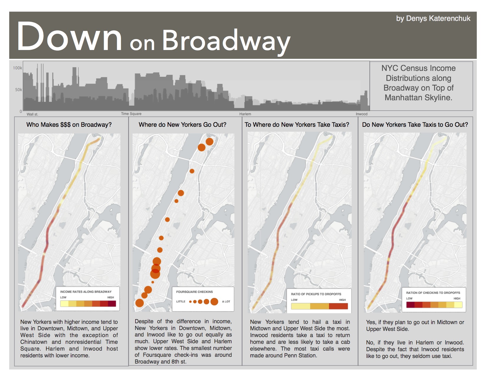
In one of the assignments, we investigated Broadway street in NYC. This is the longest street that runs through Manhattan, known for its shows, Times Square, and vibrant culture. This makes it a great source for data mining. The main areas of my investigation were income distribution and movements along this street. The data comes from different sources including the NYC census data on income change along Broadway, taxi rides, and Foursquare check-ins.
The Broadway Poster Project
The results of our Broadway analysis were compiled into a popular science style poster that combined artistic design with rigorous data analysis. The poster featured several key visualizations:
- Income Distribution Map: A choropleth map showing how income levels change along Broadway from south to north, revealing stark economic disparities across neighborhoods
- Movement Patterns: Heat maps generated from taxi ride data showing peak activity zones and times along the Broadway corridor
- Social Activity Density: Foursquare check-in data visualized as bubble charts indicating popular venues and cultural hotspots
- Temporal Analysis: Time-series plots showing how foot traffic and economic activity fluctuate throughout different hours and days
The poster design followed principles of information design, using color schemes that were both aesthetically pleasing and functionally clear. We employed a combination of warm colors for high-activity areas and cool colors for low-activity zones, making the data immediately interpretable to viewers.
Why R for Data Visualization?
The main language for this course was R, and for good reason. R is specifically designed for statistical computing and data analysis, making it an ideal choice for data visualization projects. Here are some key advantages of using R:
Core Strengths of R:
- Statistical Foundation: Built by statisticians for statisticians, with comprehensive statistical functions
- Extensive Package Ecosystem: Over 18,000 packages available on CRAN for specialized analyses
- Grammar of Graphics: The ggplot2 package implements Leland Wilkinson’s “Grammar of Graphics” philosophy
- Reproducible Research: R Markdown allows seamless integration of code, results, and documentation
- Active Community: Large, supportive community with extensive documentation and tutorials
ggplot2: The Visualization Powerhouse
The ggplot2 package is based on the “Grammar of Graphics” concept, which breaks down visualizations into layered components:
- Data: The dataset being visualized
- Aesthetics: How variables map to visual properties (x, y, color, size)
- Geometries: The type of plot (points, lines, bars)
- Facets: Subplots based on categorical variables
- Statistics: Statistical transformations of the data
- Coordinates: The coordinate system
- Themes: Overall visual styling
Useful Data Visualization Functions
Here is a comprehensive list of useful visualization techniques for anyone getting started with R:
- Bar Charts - Categorical comparisons
- Line Graphs - Trends over time
- Scatter Plots - Relationships between variables
- Heat Maps - Data density and patterns
- Box Plots - Distribution summaries
- Histograms - Frequency distributions
Bar Charts
Bar charts are useful for comparing quantities corresponding to different groups. In our Broadway analysis, we used bar charts to compare foot traffic across different subway stations along Broadway.
# R code for generating bar charts
library(ggplot2)
library(dplyr)

# Load and prepare Broadway data
broadway_data <- read.csv("broadway_stations.csv")

# Create a bar chart with custom styling
ggplot(broadway_data, aes(x = reorder(station_name, -foot_traffic), y = foot_traffic)) +
  geom_bar(stat = "identity", fill = "steelblue", alpha = 0.7) +
  coord_flip() +
  labs(title = "Foot Traffic by Broadway Subway Stations",
       subtitle = "Average daily pedestrian count",
       x = "Station Name",
       y = "Daily Foot Traffic") +
  theme_minimal() +
  theme(plot.title = element_text(size = 16, face = "bold"))
Line Graphs
Line graphs are ideal for showing trends over time. In our study, we used line graphs to display how economic indicators changed along Broadway from 2000 to 2014.
# R code for generating line graphs with multiple series
ggplot(broadway_time_series, aes(x = year, y = median_income, color = neighborhood)) +
  geom_line(size = 1.2) +
  geom_point(size = 2) +
  labs(title = "Median Income Trends Along Broadway (2000-2014)",
       x = "Year",
       y = "Median Income ($)",
       color = "Neighborhood") +
  scale_y_continuous(labels = scales::dollar_format()) +
  theme_minimal() +
  theme(legend.position = "bottom")
Scatter Plots
Scatter plots help in understanding the relationship between two quantitative variables. We used scatter plots to explore the correlation between rent prices and distance from Times Square.
# R code for generating scatter plots with regression line
ggplot(broadway_rent_data, aes(x = distance_from_times_square, y = average_rent)) +
  geom_point(alpha = 0.6, size = 2) +
  geom_smooth(method = "lm", se = TRUE, color = "red") +
  labs(title = "Rent Prices vs Distance from Times Square",
       x = "Distance from Times Square (miles)",
       y = "Average Monthly Rent ($)") +
  scale_y_continuous(labels = scales::dollar_format()) +
  theme_minimal()
Heat Maps
Heat maps are excellent for visualizing data density or intensity patterns. We created heat maps to show the concentration of Foursquare check-ins throughout different times and locations.
# R code for generating heat maps
ggplot(foursquare_data, aes(x = hour_of_day, y = day_of_week)) +
  geom_tile(aes(fill = checkin_count)) +
  scale_fill_gradient2(low = "white", mid = "yellow", high = "red",
                       midpoint = median(foursquare_data$checkin_count)) +
  labs(title = "Foursquare Check-in Density Along Broadway",
       x = "Hour of Day",
       y = "Day of Week",
       fill = "Check-ins") +
  theme_minimal() +
  theme(axis.text.x = element_text(angle = 45, hjust = 1))
Advanced Visualization Techniques
For the Broadway poster, we also employed several advanced techniques:
Faceting for Multiple Comparisons
# Create small multiples for different neighborhoods
ggplot(broadway_data, aes(x = time, y = activity_level)) +
  geom_line() +
  facet_wrap(~neighborhood, scales = "free_y") +
  labs(title = "Activity Patterns by Broadway Neighborhood") +
  theme_minimal()
Custom Color Palettes
# Define custom colors that match poster design
broadway_colors <- c("#FF6B35", "#004E89", "#F18F01", "#C73E1D")

ggplot(data, aes(x = variable, y = value, fill = category)) +
  geom_bar(stat = "identity") +
  scale_fill_manual(values = broadway_colors) +
  theme_minimal()
Conclusion
Data visualization is a powerful tool for gaining insights from complex datasets. Through our Broadway analysis, we demonstrated how R and ggplot2 can transform raw data into compelling visual narratives. The combination of statistical rigor and artistic design principles resulted in a poster that was both scientifically accurate and visually engaging.
Key takeaways from this project:
- R provides unmatched flexibility for statistical visualization
- The grammar of graphics approach makes complex visualizations more systematic
- Combining multiple data sources enriches the analytical narrative
- Good design principles are essential for effective data communication
Learning Resources
For those interested in diving deeper into R and data visualization:
Books:
- “R for Data Science” by Hadley Wickham
- “ggplot2: Elegant Graphics for Data Analysis” by Hadley Wickham
- “The Grammar of Graphics” by Leland Wilkinson